Model Evaluation

1. Loading packages and cleaned data

# load packages
library(tidyverse)

── Attaching core tidyverse packages ──────────────────────── tidyverse 2.0.0 ──
✔ dplyr     1.1.0     ✔ readr     2.1.4
✔ forcats   1.0.0     ✔ stringr   1.5.0
✔ ggplot2   3.4.1     ✔ tibble    3.1.8
✔ lubridate 1.9.2     ✔ tidyr     1.3.0
✔ purrr     1.0.1     
── Conflicts ────────────────────────────────────────── tidyverse_conflicts() ──
✖ dplyr::filter() masks stats::filter()
✖ dplyr::lag()    masks stats::lag()
ℹ Use the conflicted package (<http://conflicted.r-lib.org/>) to force all conflicts to become errors

library(here)

here() starts at C:/Users/Katie/Documents/2022-2023/MADA/katiewells-MADA-portfolio

library(tidymodels)

── Attaching packages ────────────────────────────────────── tidymodels 1.0.0 ──
✔ broom        1.0.3     ✔ rsample      1.1.1
✔ dials        1.1.0     ✔ tune         1.0.1
✔ infer        1.0.4     ✔ workflows    1.1.3
✔ modeldata    1.1.0     ✔ workflowsets 1.0.0
✔ parsnip      1.0.4     ✔ yardstick    1.1.0
✔ recipes      1.0.5     
── Conflicts ───────────────────────────────────────── tidymodels_conflicts() ──
✖ scales::discard() masks purrr::discard()
✖ dplyr::filter()   masks stats::filter()
✖ recipes::fixed()  masks stringr::fixed()
✖ dplyr::lag()      masks stats::lag()
✖ yardstick::spec() masks readr::spec()
✖ recipes::step()   masks stats::step()
• Learn how to get started at https://www.tidymodels.org/start/

# load cleaned data
flu2 <- readRDS(here("fluanalysis", "data", "flu2.rds"))

2. Split data

set.seed(222)
# Put 3/4 of the data into the training set 
data_split <- initial_split(flu2, prop = 3/4)

# Create data frames for the two sets:
train_data <- training(data_split)
test_data  <- testing(data_split)

3. Create recipe

flu_rec <- 
  recipe(Nausea ~ ., data = train_data) 

4. Fit model with recipe

#setting logistic regression engine
lr_mod <- 
  logistic_reg() %>% 
  set_engine("glm")

#creating workflow using model and recipe
flu_wflow <- 
  workflow() %>% 
  add_model(lr_mod) %>% 
  add_recipe(flu_rec)
flu_wflow

══ Workflow ════════════════════════════════════════════════════════════════════
Preprocessor: Recipe
Model: logistic_reg()

── Preprocessor ────────────────────────────────────────────────────────────────
0 Recipe Steps

── Model ───────────────────────────────────────────────────────────────────────
Logistic Regression Model Specification (classification)

Computational engine: glm 

#make function to prepare the recipe and train the model 
flu_fit <- 
  flu_wflow %>% 
  fit(data = train_data)

#pull fitting model object and make tibble of model coefficients
flu_fit %>% 
  extract_fit_parsnip() %>% 
  tidy()

# A tibble: 32 × 5
   term                 estimate std.error statistic p.value
   <chr>                   <dbl>     <dbl>     <dbl>   <dbl>
 1 (Intercept)            2.56       9.39      0.273  0.785 
 2 SwollenLymphNodesYes  -0.240      0.231    -1.04   0.300 
 3 ChestCongestionYes     0.168      0.252     0.668  0.504 
 4 ChillsSweatsYes        0.148      0.331     0.448  0.654 
 5 NasalCongestionYes     0.600      0.309     1.94   0.0521
 6 SneezeYes              0.0974     0.247     0.395  0.693 
 7 FatigueYes             0.180      0.438     0.411  0.681 
 8 SubjectiveFeverYes     0.191      0.261     0.733  0.463 
 9 HeadacheYes            0.482      0.351     1.37   0.169 
10 Weakness.L             0.668      0.406     1.65   0.0999
# … with 22 more rows

5. Using trained workflow to predict (test data)

#use trained model to predict with unseen data
predict(flu_fit, test_data)

# A tibble: 183 × 1
   .pred_class
   <fct>      
 1 No         
 2 No         
 3 No         
 4 No         
 5 No         
 6 Yes        
 7 Yes        
 8 No         
 9 No         
10 Yes        
# … with 173 more rows

#save above together to use to get ROC
flu_aug <- 
  augment(flu_fit, test_data)

#view the data
flu_aug %>%
  select(Nausea, .pred_No, .pred_Yes)

# A tibble: 183 × 3
   Nausea .pred_No .pred_Yes
   <fct>     <dbl>     <dbl>
 1 No        0.962    0.0377
 2 Yes       0.708    0.292 
 3 No        0.696    0.304 
 4 Yes       0.548    0.452 
 5 No        0.826    0.174 
 6 Yes       0.193    0.807 
 7 Yes       0.227    0.773 
 8 No        0.712    0.288 
 9 No        0.688    0.312 
10 Yes       0.271    0.729 
# … with 173 more rows

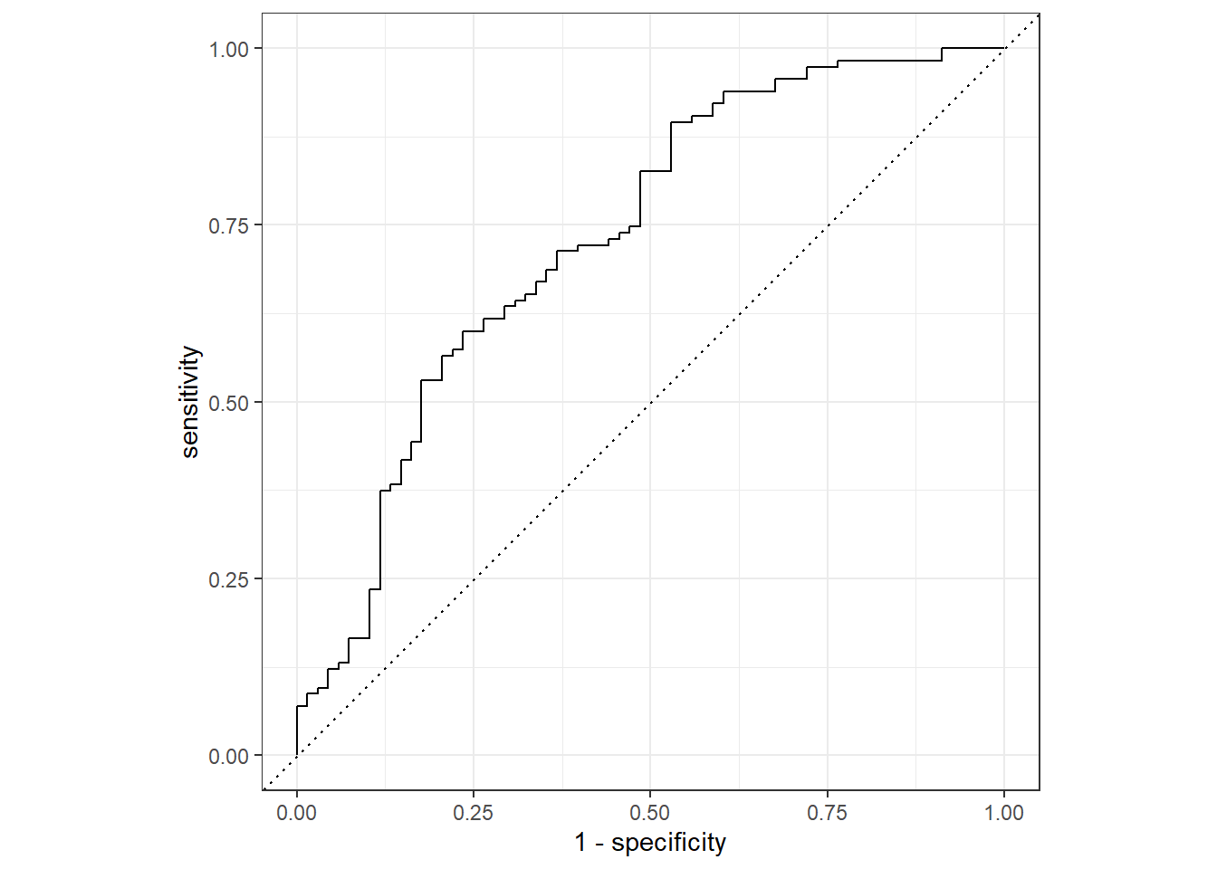
#create ROC curve with predicted class probabilities 
flu_aug %>% 
  roc_curve(truth = Nausea, .pred_No) %>% 
  autoplot()

Warning: Returning more (or less) than 1 row per `summarise()` group was deprecated in
dplyr 1.1.0.
ℹ Please use `reframe()` instead.
ℹ When switching from `summarise()` to `reframe()`, remember that `reframe()`
  always returns an ungrouped data frame and adjust accordingly.
ℹ The deprecated feature was likely used in the yardstick package.
  Please report the issue at <https://github.com/tidymodels/yardstick/issues>.

#ROC estimate
flu_aug %>% 
  roc_auc(truth = Nausea, .pred_No) 

# A tibble: 1 × 3
  .metric .estimator .estimate
  <chr>   <chr>          <dbl>
1 roc_auc binary         0.731

Refitting with the main predicotr (RunnyNose) and using the trained model to predict with test and train data.

7. Alternative Model

flu_rec2 <- 
  recipe(Nausea ~ RunnyNose, data = train_data) 

flu_wflow2 <- 
  workflow() %>% 
  add_model(lr_mod) %>% 
  add_recipe(flu_rec2)
flu_wflow2

══ Workflow ════════════════════════════════════════════════════════════════════
Preprocessor: Recipe
Model: logistic_reg()

── Preprocessor ────────────────────────────────────────────────────────────────
0 Recipe Steps

── Model ───────────────────────────────────────────────────────────────────────
Logistic Regression Model Specification (classification)

Computational engine: glm 

flu_fit2 <- 
  flu_wflow2 %>% 
  fit(data = train_data)

flu_fit2 %>% 
  extract_fit_parsnip() %>% 
  tidy()

# A tibble: 2 × 5
  term         estimate std.error statistic    p.value
  <chr>           <dbl>     <dbl>     <dbl>      <dbl>
1 (Intercept)    -0.790     0.172    -4.59  0.00000447
2 RunnyNoseYes    0.188     0.202     0.930 0.352     

8. Using trained workflow to predict (test data)

predict(flu_fit2, test_data)

# A tibble: 183 × 1
   .pred_class
   <fct>      
 1 No         
 2 No         
 3 No         
 4 No         
 5 No         
 6 No         
 7 No         
 8 No         
 9 No         
10 No         
# … with 173 more rows

flu_aug3 <- 
  augment(flu_fit2, test_data)

flu_aug3 %>%
  select(Nausea, .pred_No, .pred_Yes)

# A tibble: 183 × 3
   Nausea .pred_No .pred_Yes
   <fct>     <dbl>     <dbl>
 1 No        0.688     0.312
 2 Yes       0.646     0.354
 3 No        0.646     0.354
 4 Yes       0.646     0.354
 5 No        0.688     0.312
 6 Yes       0.688     0.312
 7 Yes       0.646     0.354
 8 No        0.688     0.312
 9 No        0.688     0.312
10 Yes       0.688     0.312
# … with 173 more rows

flu_aug3 %>% 
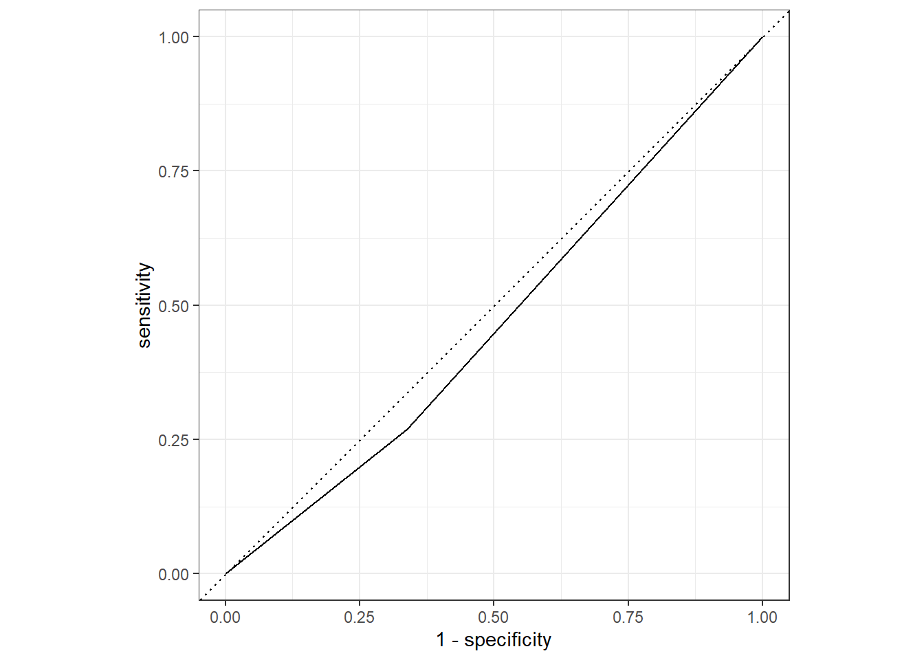
  roc_curve(truth = Nausea, .pred_No) %>% 
  autoplot()

flu_aug3 %>% 
  roc_auc(truth = Nausea, .pred_No) 

# A tibble: 1 × 3
  .metric .estimator .estimate
  <chr>   <chr>          <dbl>
1 roc_auc binary         0.466

The model using only runny nose as a predictor had a lower ROC than the model with all predictors.

This section added by Hayley Hemme

9. Create recipe

flu_ln_rec <- 
  recipe(BodyTemp ~ ., data = train_data) 

10. Fit linear model

#setting linear regression engine
ln_mod <- 
  linear_reg() %>% 
  set_engine("lm") %>% 
  set_mode("regression")

#creating workflow using model and recipe
flu_ln_wflow <- 
  workflow() %>% 
  add_model(ln_mod) %>% 
  add_recipe(flu_ln_rec)

#make function to prepare the recipe and train the model 
flu_ln_fit <- 
  flu_ln_wflow %>% 
  fit(data = train_data)

#pull fitting model object and make tibble of model coefficients
flu_ln_fit %>% 
  extract_fit_parsnip() %>% 
  tidy()

# A tibble: 32 × 5
   term                 estimate std.error statistic    p.value
   <chr>                   <dbl>     <dbl>     <dbl>      <dbl>
 1 (Intercept)           98.0        0.280   350.    0         
 2 SwollenLymphNodesYes  -0.190      0.108    -1.76  0.0789    
 3 ChestCongestionYes     0.146      0.115     1.27  0.203     
 4 ChillsSweatsYes        0.184      0.148     1.24  0.214     
 5 NasalCongestionYes    -0.182      0.136    -1.34  0.180     
 6 SneezeYes             -0.474      0.113    -4.18  0.0000338 
 7 FatigueYes             0.362      0.187     1.94  0.0529    
 8 SubjectiveFeverYes     0.564      0.118     4.79  0.00000223
 9 HeadacheYes            0.0675     0.150     0.448 0.654     
10 Weakness.L             0.224      0.182     1.23  0.218     
# … with 22 more rows

10. Using trained workflow to predict (test data)

#use trained model to predict with unseen data
predict(flu_ln_fit, test_data)

# A tibble: 183 × 1
   .pred
   <dbl>
 1  99.4
 2  99.0
 3  99.8
 4  98.7
 5  99.0
 6  99.6
 7  99.2
 8  98.8
 9  99.5
10  98.8
# … with 173 more rows

#save above together 
flu_ln_aug <- 
  augment(flu_ln_fit, test_data)

#view the data
flu_ln_aug %>%
  select(BodyTemp, .pred)

# A tibble: 183 × 2
   BodyTemp .pred
      <dbl> <dbl>
 1     98.3  99.4
 2     98.8  99.0
 3    102.   99.8
 4     98.2  98.7
 5     97.8  99.0
 6     97.8  99.6
 7    100    99.2
 8    101.   98.8
 9     98.8  99.5
10    100.   98.8
# … with 173 more rows

Measuring model fit - RMSE

flu_ln_aug %>%
  rmse(truth = BodyTemp, .pred)

# A tibble: 1 × 3
  .metric .estimator .estimate
  <chr>   <chr>          <dbl>
1 rmse    standard        1.15

Let’s also measure model fit using R2

flu_ln_aug %>% 
  rsq(truth = BodyTemp, .pred) 

# A tibble: 1 × 3
  .metric .estimator .estimate
  <chr>   <chr>          <dbl>
1 rsq     standard      0.0446

Making a plot using predictions

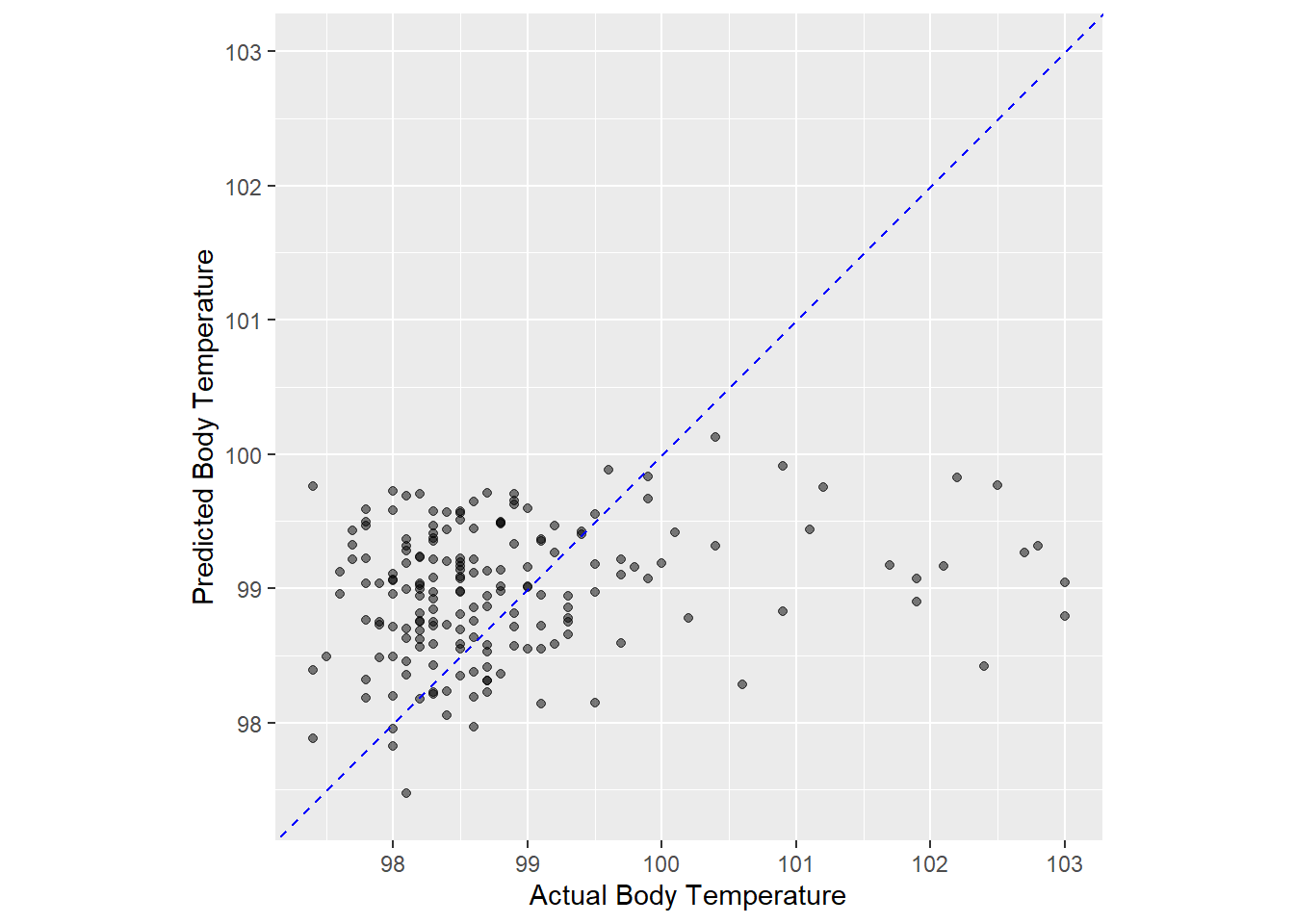
ggplot(flu_ln_aug, aes(x = BodyTemp, y = .pred)) +
  geom_point(alpha = 0.5) + 
  geom_abline(color = 'blue', linetype = 2) +
  coord_obs_pred() +
  labs(x = 'Actual Body Temperature', y = 'Predicted Body Temperature')

This trained model is not very well suited to predict body temperature using all the predictors in the model. Let move on and…

Refit with the main predictor (RunnyNose) and use the trained model to predict with test and train data. 11. Alternative Model Creating recipe

flu_ln_rec2 <- 
  recipe(BodyTemp ~ RunnyNose, data = train_data) 

Making workflow object

flu_ln_wflow2 <- 
  workflow() %>% 
  add_model(ln_mod) %>% 
  add_recipe(flu_ln_rec2)

Making fit object

flu_ln_fit2 <- 
  flu_ln_wflow2 %>% 
  fit(data = train_data)

Extracting data of the model fit

flu_ln_fit2 %>% 
  extract_fit_parsnip() %>% 
  tidy()

# A tibble: 2 × 5
  term         estimate std.error statistic p.value
  <chr>           <dbl>     <dbl>     <dbl>   <dbl>
1 (Intercept)    99.1      0.0964   1028.    0     
2 RunnyNoseYes   -0.261    0.114      -2.29  0.0225

12. Using trained workflow to predict (test data)

predict(flu_ln_fit2, test_data)

# A tibble: 183 × 1
   .pred
   <dbl>
 1  99.1
 2  98.9
 3  98.9
 4  98.9
 5  99.1
 6  99.1
 7  98.9
 8  99.1
 9  99.1
10  99.1
# … with 173 more rows

flu_ln_aug3 <- 
  augment(flu_ln_fit2, test_data)

flu_ln_aug3 %>%
  select(BodyTemp, .pred)

# A tibble: 183 × 2
   BodyTemp .pred
      <dbl> <dbl>
 1     98.3  99.1
 2     98.8  98.9
 3    102.   98.9
 4     98.2  98.9
 5     97.8  99.1
 6     97.8  99.1
 7    100    98.9
 8    101.   99.1
 9     98.8  99.1
10    100.   99.1
# … with 173 more rows

Measuring model fit - RMSE

flu_ln_aug3 %>%
  rmse(truth = BodyTemp, .pred)

# A tibble: 1 × 3
  .metric .estimator .estimate
  <chr>   <chr>          <dbl>
1 rmse    standard        1.13

Let’s also measure model fit using R2

flu_ln_aug3 %>% 
  rsq(truth = BodyTemp, .pred) 

# A tibble: 1 × 3
  .metric .estimator .estimate
  <chr>   <chr>          <dbl>
1 rsq     standard      0.0240

Make an R2 plot using predictions

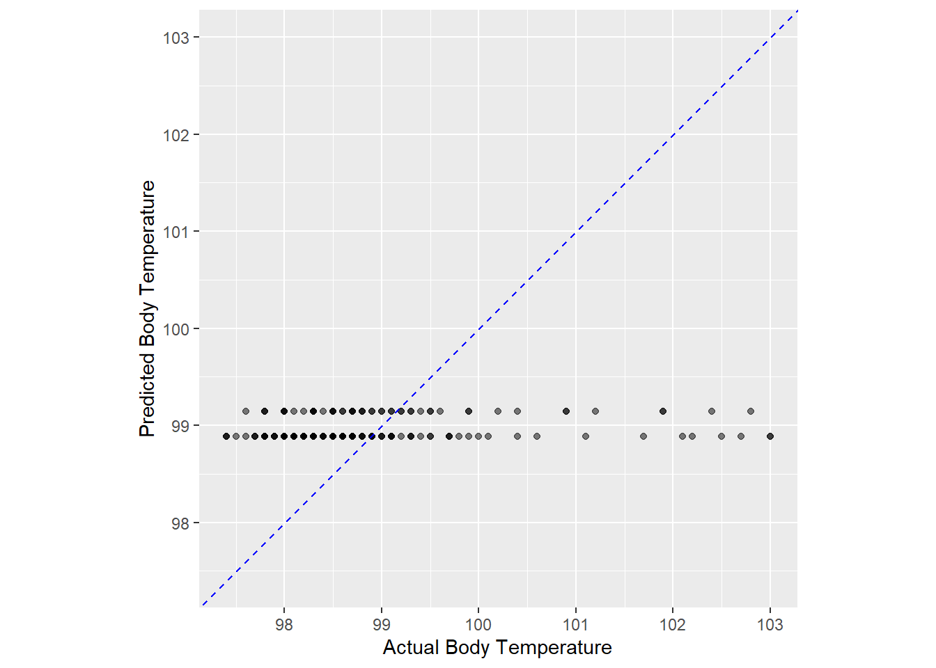
ggplot(flu_ln_aug3, aes(x = BodyTemp, y = .pred)) +
  geom_point(alpha = 0.5) + 
  geom_abline(color = 'blue', linetype = 2) +
  coord_obs_pred() +
  labs(x = 'Actual Body Temperature', y = 'Predicted Body Temperature')

The model preformed very poorly using runny nose as predictor of body temperature. I am also wondering why the model only had two different predictions, and makes me think that something may have went wrong with setting up the model?